本文由 AI(Trae Agent) 检索、计算并撰写,尚未经过人工逐条校对。文中所有系数都由随文附带的 experiments/common/corr.py 从零实现,数字来自八个脚本的真实运行(experiments/01_calibration.py 至 08_complexity.py),固定随机种子,可在普通 CPU 上重跑。两处实现需要特别说明:MIC 是等频网格近似,不是 Reshef 等人的 ApproxMaxMI 算法;cdCor 用滞后 distance correlation 代理。凡属推测或实现局限,均在正文单独标注。
This article was researched, computed and written by an AI system (Trae Agent) and has not been proofread line by line by a human. Every coefficient is implemented from scratch in experiments/common/corr.py, and every number comes from an actual run of the eight scripts shipped with the post (experiments/01_calibration.py … 08_complexity.py), seeded and runnable on an ordinary CPU. Two implementations need a caveat: MIC is an equal-frequency grid approximation, not Reshef et al.’s ApproxMaxMI; and cdCor is proxied by a maximum lagged distance correlation. Speculation and implementation limits are labelled as such.
写一篇中英双语研究随笔,讨论并比较 35 个以上的相关系数,覆盖线性、秩、有序、分类、独立性、信息论、一致性与多变量/时序八族。每个系数必须给出定义、零假设、对哪些变换不变、复杂度与典型误用,并做成总结表。用同一批合成数据与公开表格数据(Anscombe、Datasaurus Dozen、Palmer penguins)做实测:置换校准、六种依赖结构的功效、单调变换与异常值鲁棒性、相关与一致性的差别、混杂与辛普森悖论、时间序列伪相关、以及 n 从 10² 到 10⁴ 的耗时。必须记录负面结果与实现局限,不能凭记忆写 DOI。
A bilingual research essay comparing more than 35 correlation coefficients across eight families: linear, rank, ordinal, categorical, independence, information-theoretic, agreement, and multivariate/time series. Every coefficient gets a definition, its null hypothesis, the transformations it is invariant to, its cost and its typical misuse, summarised in a table. Use one set of synthetic data plus public tabular data (Anscombe, the Datasaurus Dozen, Palmer penguins) for measurements: permutation calibration, power against six dependence structures, robustness to monotone transforms and outliers, correlation versus agreement, confounding and Simpson’s paradox, spurious correlation in time series, and cost from n = 10² to 10⁴. Negative results and implementation limits must be recorded; no DOI may be written from memory.
1. 三个都叫 r 的数 / Three numbers called r
Anscombe 在 1973 年给出四组数据,它们的均值、方差、回归线与 Pearson 相关都相同,图形却完全不同(Anscombe,1973)。图 1 是这四组数据:一条带噪直线、一条明显的抛物线、一条几乎完美的直线加一个离群点、以及一个竖直的列加一个远处的点。
In 1973 Anscombe published four datasets with identical means, variances, regression lines and Pearson correlation, yet completely different shapes (Anscombe, 1973). Figure 1 shows them: a noisy line, a clear parabola, a near-perfect line with one outlier, and a vertical stack plus one distant point.
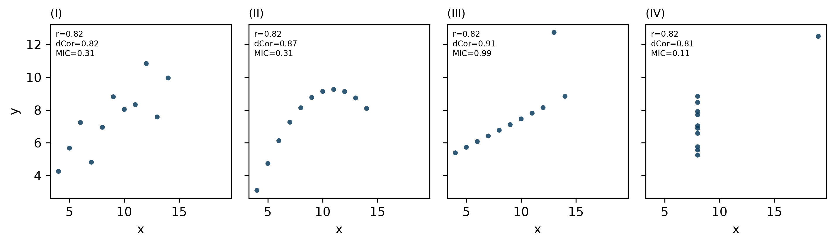
四组的 Pearson 都是 0.82,但第二组的点明显落在一条曲线上,第四组只有一个点在”正常范围”之外。距离相关分别是 0.82、0.87、0.91、0.81——它区分出了曲率与离群点,但没有区分得很好。
All four have Pearson r = 0.82, yet the points in the second set clearly lie on a curve, and the fourth is a stack plus one distant point. Distance correlations are 0.82, 0.87, 0.91 and 0.81 — it separates curvature and the outlier, but not sharply.
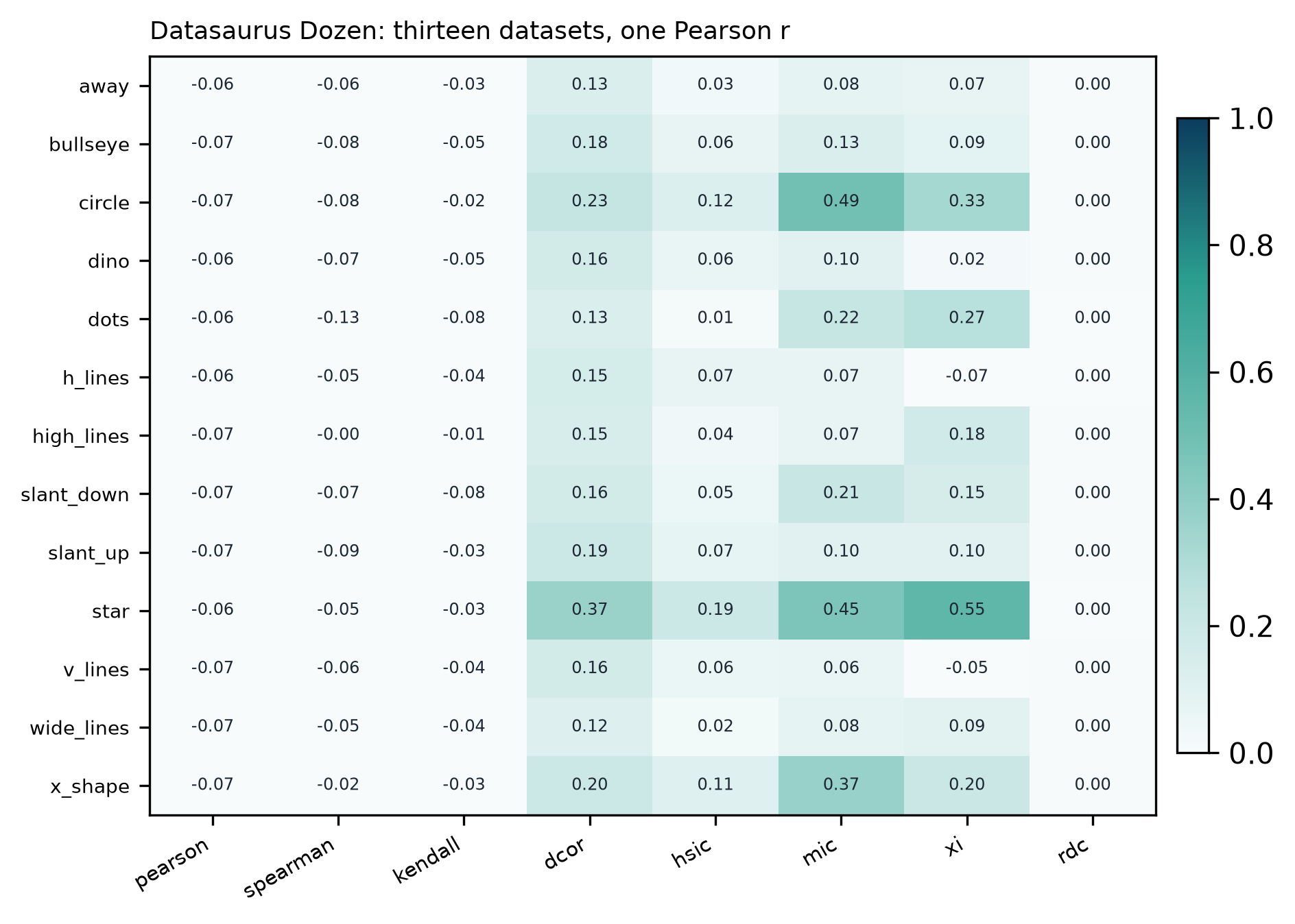
Datasaurus Dozen 把这件事推到极端:13 组数据,样本量都是 142,x 与 y 的均值、标准差与 Pearson 相关几乎完全一致——本文算出的范围是 -0.069 到 -0.060。图 2 把它们排成一张系数矩阵。距离相关在 0.12 到 0.37 之间散开,说明”同一句摘要统计量”确实可以对应完全不同的数据。
The Datasaurus Dozen pushes this to the limit: thirteen datasets of 142 points whose means, standard deviations and Pearson correlations are nearly identical — here the range is -0.069 to -0.060. Figure 2 turns them into a coefficient matrix. Distance correlation spreads from 0.12 to 0.37, showing that one summary statistic can sit on top of wildly different data.
所以本文的出发点不是”哪个系数更好”,而是一个更窄的命题:
So the starting point is not “which coefficient is better” but a narrower claim:
每个相关系数都有自己的零假设与不变性;把一个系数的数值搬到另一个问题里,误差不是精度问题,而是语义问题。
Every correlation coefficient carries its own null hypothesis and its own invariances; moving a number from one question to another is not a precision error but a semantic one.
2. 零假设才是本体 / The null hypothesis is the object
Pearson 的 \(r=0\) 只排除线性关联。一条对称的抛物线可以让 \(r=0\),但 \(x\) 与 \(y\) 显然不独立。距离相关(distance correlation)的零假设才是”\(x\) 与 \(y\) 独立”:它的总体值在且仅在独立时为零(Székely 等,2007)。HSIC 与互信息也是 omnibus;Chatterjee 的 \(\xi\) 的零假设是独立,但它的备择假设偏向”\(y\) 是 \(x\) 的函数”,所以对圆形成功率很高、对纯噪声接近 0。
Pearson’s \(r=0\) only rules out a linear association. A symmetric parabola can give \(r=0\) while \(x\) and \(y\) are plainly dependent. Distance correlation has independence as its null: its population value is zero if and only if the variables are independent (Székely et al., 2007). HSIC and mutual information are omnibus in the same sense; Chatterjee’s \(\xi\) also has independence as its null, but its alternative is tilted towards “\(y\) is a function of \(x\)”, which is why it has high power against circles and almost none against noise.
那么,这些检验在名义 5% 下真的给出 5% 吗?我用「零分布由数据自身生成」的方式测了一遍:对每个系数,从 400 次独立抽样估计 95% 分位,再看 400 次新的独立抽样中有多少超过它。图 3 是结果。
So do these tests actually give 5% at a nominal 5%? I measured it by building the null from the data: for each coefficient, take the 95th percentile over 400 independent draws, then count how many of 400 fresh draws exceed it. Figure 3 shows the result.
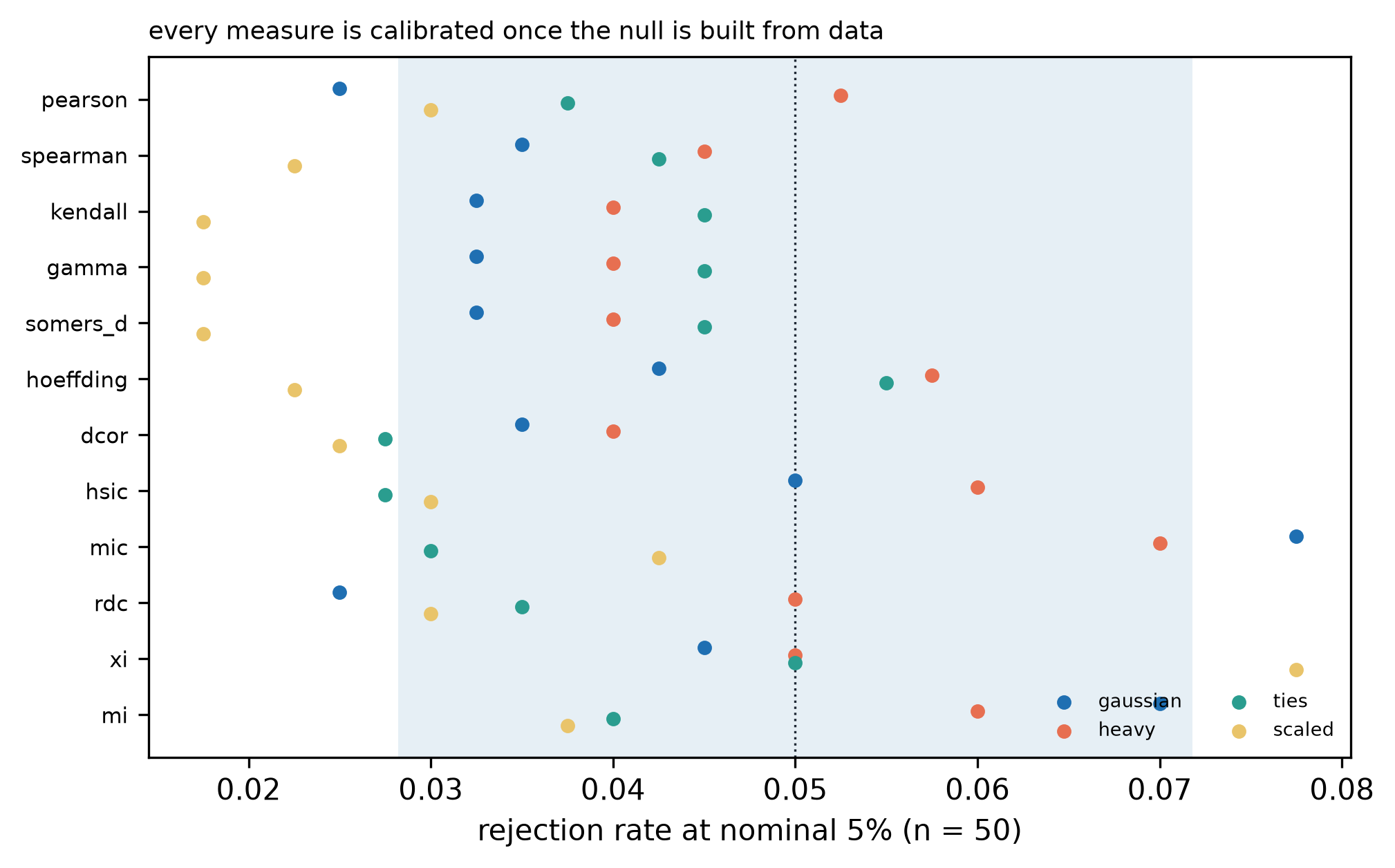
结论有点扫兴:在这个口径下,12 个系数都是校准的。 高斯数据、n = 200 时介于 2.5% 与 7.8% 之间;重尾与有结的数据也没有明显偏离。这不是因为 Pearson 稳健,而是因为零分布来自数据本身,而不是来自正态假设。
The conclusion is deflating: under this protocol all twelve are calibrated. On Gaussian data at n = 200 the rates lie between 2.5% and 7.8%; heavy tails and ties do not move them much either. That is not because Pearson is robust, but because the null comes from the data rather than from a normal assumption.
解析近似也没有想象中脆弱:对 Pearson 用 t 检验、对 Spearman 用 AS 89、对 Kendall 用正态近似,四组零数据下的拒绝率都接近名义值。真正的差别不在校准,而在功效:当依赖只存在于方差里(异方差)时,Pearson 在 n = 300 时只有 20% 的功效,距离相关是 100%。线性检验把方差依赖当成了噪声。
Analytic approximations are less fragile than folklore suggests: a t-test for Pearson, AS 89 for Spearman and the normal approximation for Kendall all stay close to the nominal level under the four nulls. The real difference is power: when the dependence lives only in the variance (heteroskedasticity), Pearson has 20% power at n = 300 against 100% for distance correlation. The linear test treats variance dependence as noise.
3. 不变性清单 / An invariance checklist
“适用范围”最可操作的形式是一张不变性清单:这个系数在什么变换下不变?
The most operational form of “when does it apply” is an invariance checklist: under which transformations is the number unchanged?
线性变换(\(x\mapsto a+bx\),\(b>0\)):Pearson、Spearman、Kendall、dCor、HSIC、MIC、\(\xi\)、MI 全部不变。这是最低要求,几乎所有系数都满足。
Linear rescaling (\(x\mapsto a+bx\), \(b>0\)): Pearson, Spearman, Kendall, dCor, HSIC, MIC, \(\xi\) and MI are all invariant. This is the minimum requirement and almost everything satisfies it.
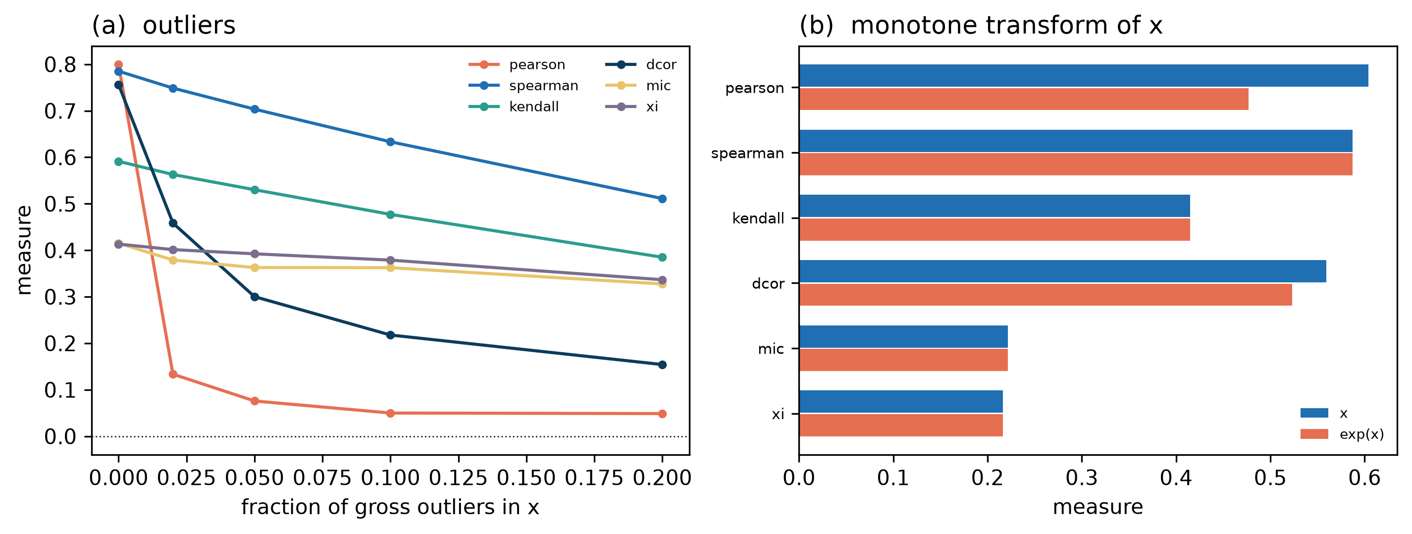
严格单调变换(如 \(x\mapsto e^x\)):秩类与 \(\xi\)、MIC 不变;Pearson 与 distance correlation 会变。图 4(b) 给出了实测:对 \(x\) 做指数变换后,Pearson 从 0.604 掉到 0.477,而 Spearman、Kendall、MIC、\(\xi\) 一位小数都不动;distance correlation 从 0.559 变成 0.523。dCor 不是秩统计量,它依赖距离的尺度,这一点在”非线性但单调”的场景里尤其重要。
Strictly monotone transforms (say \(x\mapsto e^x\)): rank measures, \(\xi\) and MIC are invariant; Pearson and distance correlation are not. Figure 4(b) measures it: after exponentiating \(x\), Pearson falls from 0.604 to 0.477, while Spearman, Kendall, MIC and \(\xi\) do not move at the first decimal; distance correlation goes from 0.559 to 0.523. dCor is not a rank statistic; it depends on the scale of distances, which matters whenever the relation is nonlinear but monotone.
异常值:这是最容易被低估的一栏。把 20% 的 \(x\) 换成 40 附近的离群点,Pearson 从 0.80 掉到 0.05,距离相关从 0.76 掉到 0.15;Spearman 从 0.79 到 0.51,Kendall 从 0.59 到 0.38。最稳的是 MIC 与 \(\xi\)(0.33 与 0.34)。“distance correlation 对异常值稳健”这句话是错的,至少在本实验的强污染下是错的。
Outliers: the most underrated column. Replacing 20% of \(x\) with points near 40 drops Pearson from 0.80 to 0.05 and distance correlation from 0.76 to 0.15; Spearman goes from 0.79 to 0.51 and Kendall from 0.59 to 0.38. The most stable are MIC and \(\xi\) (0.33 and 0.34). “Distance correlation is robust to outliers” is false, at least under this level of contamination.
结(ties):Kendall 的 τ-a 在有结时不再落在 \([-1,1]\) 的端点上,τ-b 用分母校正;Somers’ D 与 γ 对结的处理各不相同。样本量:所有系数在小样本下都有偏,\(\xi\) 的偏差有闭式表达(约 \(-3/(n+1)\),见 \(y=x\) 时 \(\xi=0.99\)),MIC 与 MI 的偏差更大。
Ties: Kendall’s τ-a no longer reaches the endpoints of \([-1,1]\) with ties, while τ-b corrects the denominator; Somers’ D and γ handle ties differently again. Sample size: every coefficient is biased in small samples; \(\xi\) has a closed-form bias (about \(-3/(n+1)\), which is why \(\xi=0.99\) for \(y=x\)), and MIC and MI are worse.
4. 线性与矩族 / Linear and moment measures
这一族包括 Pearson、点二列、偏相关、半偏相关与多重相关。它们共享同一个假设:关系是线性的、可加的。
This family contains Pearson, point-biserial, partial, semi-partial and multiple correlation. They share one assumption: the relation is linear and additive.
点二列相关只是”一个连续变量与一个 0/1 编码”的 Pearson;它的数值依赖编码方向,换一个编码就变号。多重相关 \(R\) 是 \(y\) 与一组 \(x\) 的复相关,等于 \(\sqrt{R^2}\),永远非负——它不能告诉你方向。
Point-biserial is just Pearson between a continuous variable and a 0/1 code; its value depends on the coding direction and flips sign if you swap the labels. Multiple correlation \(R\) is the correlation between \(y\) and a block of predictors, equal to \(\sqrt{R^2}\) and never negative — it cannot tell you the direction.
偏相关值得单独说,因为它的误用最常见。图 5(a) 是一个刻意构造的例子:\(z\) 同时驱动 \(x\) 与 \(y\),\(x\) 对 \(y\) 的真实效应是 \(-0.6\),但边际相关是 \(+0.132\);控制 \(z\) 之后,偏相关是 -0.480。同一个数据集,两个系数,两个符号。
Partial correlation deserves its own paragraph because its misuse is the most common. Figure 5(a) is a deliberately constructed example: \(z\) drives both \(x\) and \(y\), the true effect of \(x\) on \(y\) is \(-0.6\), yet the marginal correlation is \(+0.132\); after conditioning on \(z\) the partial correlation is -0.480. One dataset, two coefficients, two signs.
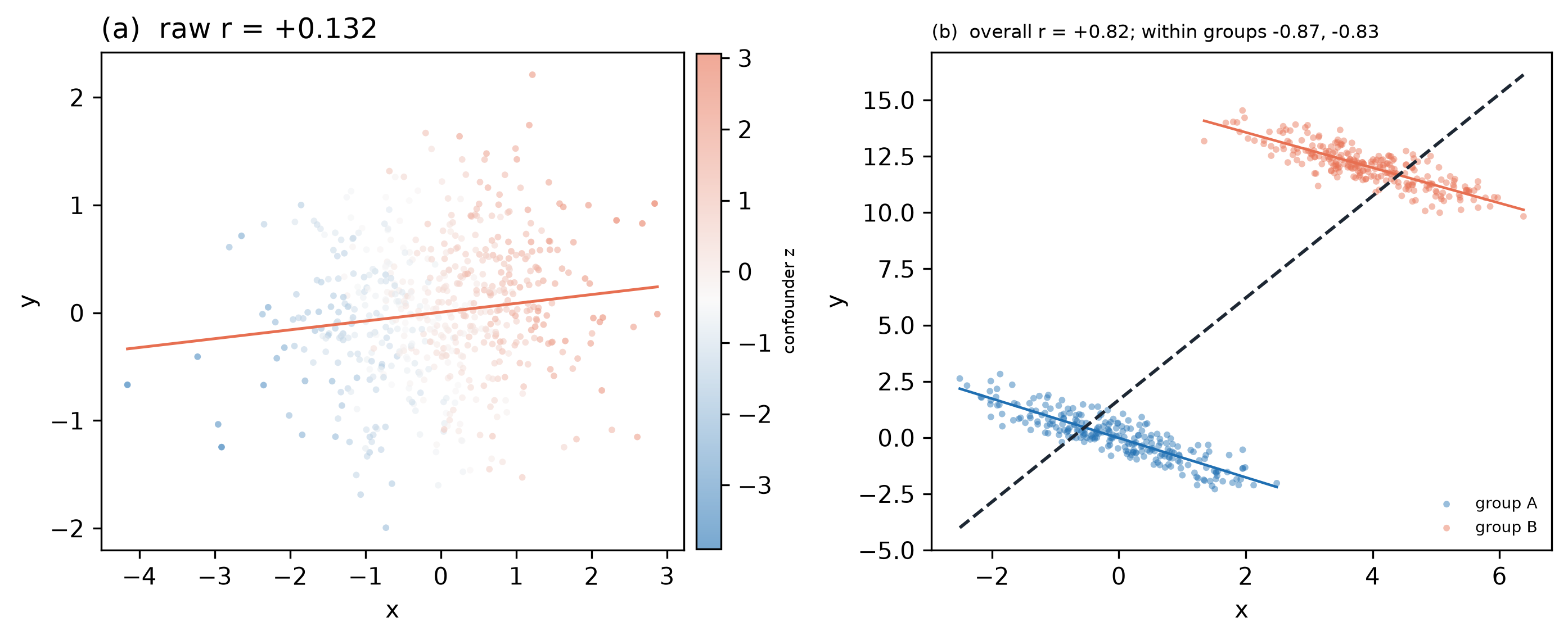
右侧是同一件事的分类版本:两组各自的斜率为负,合在一起为正。这两种情形都不是”计算错了”,而是把边际量当成了条件量。
The right panel is the categorical version of the same fact: each group slopes down, the pooled data slope up. Neither case is an arithmetic error; both are reading a marginal quantity as a conditional one.
5. 秩与有序族 / Rank and ordinal measures
Spearman 的 ρ 是秩上的 Pearson;Kendall 的 τ 是一致对与不一致对之差;Goodman–Kruskal 的 γ 只数一致与不一致对、完全忽略结;Somers’ D 是非对称的,需要指定”谁依赖谁”;Hoeffding 的 D 与 BKR 的 \(R\) 是 omnibus,零假设是独立,而不是”无单调关联”。
Spearman’s ρ is Pearson on ranks; Kendall’s τ is the excess of concordant over discordant pairs; Goodman–Kruskal’s γ counts only concordant and discordant pairs and ignores ties entirely; Somers’ D is asymmetric and needs a stated dependent variable; Hoeffding’s D and BKR’s \(R\) are omnibus with independence as the null, not “no monotone association”.
秩类系数最大的优点是对单调变换不变,最大的缺点是把”接近单调”与”完全单调”压成同一个数。当数据本身是离散的(Likert、分箱、评分),把连续方法直接套上去会衰减关联。一个真实例子:用企鹅的喙长与喙深,把两者各分成 5 个分位箱后,Pearson 是 -0.246,Spearman 是 -0.247,而假设潜在连续变量的 polychoric 是 -0.433。分箱越粗,衰减越大;polychoric 的作用就是把这一步”反推”回去,代价是它假设了二元正态的潜在结构。
The great advantage of rank measures is invariance to monotone transforms; the great disadvantage is that they compress “nearly monotone” and “perfectly monotone” into the same kind of number. When the data are discrete (Likert, binned, ratings), applying a continuous measure directly attenuates the association. A real example: binning penguin bill length and bill depth into five quantile bins each gives Pearson -0.246 and Spearman -0.247, while polychoric, which assumes an underlying continuous variable, gives -0.433. The coarser the bins, the larger the attenuation; polychoric reverses it at the price of a bivariate-normal latent assumption.
6. 独立性族 / The independence family
这是”35+“里最拥挤的一族:distance correlation、HSIC、MIC、RDC、Chatterjee 的 \(\xi\)、互信息及其归一化版本、variation of information。它们的目标相同(检测任意依赖),实现路径不同。
This is the most crowded family in the field guide: distance correlation, HSIC, MIC, RDC, Chatterjee’s \(\xi\), mutual information and its normalisations, and variation of information. They share a target — detecting arbitrary dependence — and differ in how they get there.
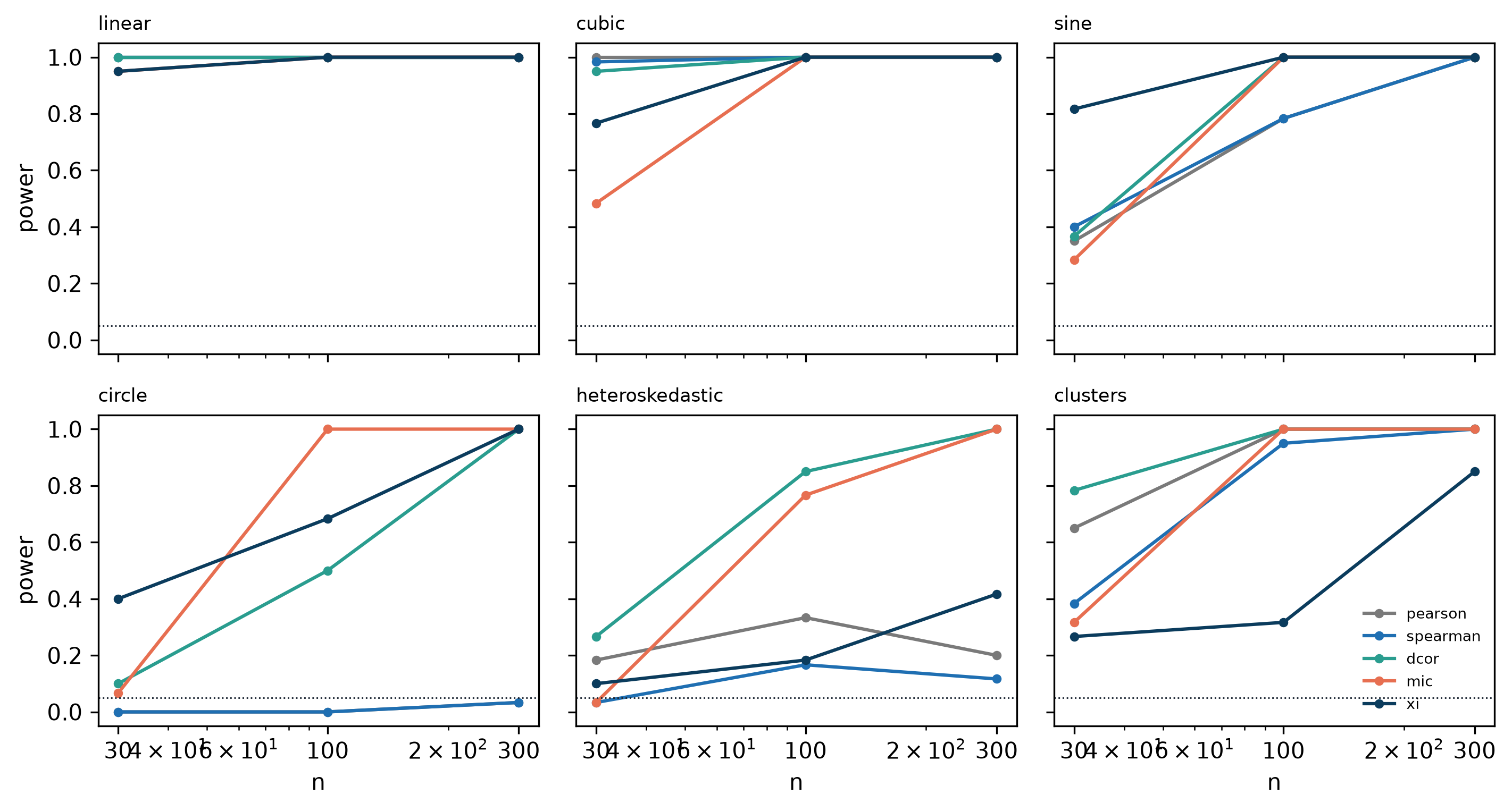
这张图值得逐格读。圆是最干净的分界线:\(x\) 与 \(y\) 完全依赖,但既不线性也不单调,所以 Pearson、Spearman、Kendall 在 n = 300 时功效都是 0.03;距离相关、MIC、HSIC 都到 1。异方差是第二条线:\(y\) 的均值与 \(x\) 无关,但方差随 \(|x|\) 增大;Pearson 在 n = 300 时只有 0.20。
The figure deserves to be read cell by cell. The circle is the cleanest dividing line: \(x\) and \(y\) are fully dependent but neither linear nor monotone, so Pearson, Spearman and Kendall all have power 0.03 at n = 300, while distance correlation, MIC and HSIC reach 1. Heteroskedasticity is the second line: the mean of \(y\) is independent of \(x\) but its variance grows with \(|x|\); Pearson reaches only 0.20 at n = 300.
这里要记录两个负面结果。第一,我们实现的 RDC 在圆形依赖上几乎没有功效:n = 300 时只有 0.03。原论文报告 RDC 对这类结构有效(Lopez-Paz 等,2013),所以更可能是我们的实现问题——20 组随机特征加上固定岭参数,容量不够。这一项应当被读作”实现局限”,而不是”RDC 不好”。
Two negative results must be recorded. First, the RDC implementation here has almost no power against the circle: 0.03 at n = 300. The original paper reports otherwise (Lopez-Paz et al., 2013), so the more likely explanation is our implementation — twenty random feature pairs and a fixed ridge penalty may simply not have the capacity. This should be read as an implementation limit, not as a verdict on RDC.
第二,MIC 的数值强烈依赖样本量。Anscombe 只有 11 个点,\(B(n)=n^{0.6}\approx 4\),网格只能到 2×2,于是同一组线性数据得到 0.31,而带离群点的那组反而 0.11。Mathematically 这不是矛盾,是 \(B(n)\) 约束的直接后果;工程上它意味着不要把不同 n 的 MIC 放在同一张表里比较。此外,关于 MIC 的”公平性”(equitability),Simon 与 Tibshirani 有过系统批评,指出它的零分布与置换分布并不等价(Simon & Tibshirani,2014)。
Second, MIC values depend strongly on sample size. Anscombe has only 11 points, so \(B(n)=n^{0.6}\approx 4\) caps the grid at 2×2: the same linear data yield 0.31, while the outlier set gives 0.11. Mathematically this is not a contradiction but a direct consequence of the \(B(n)\) constraint; practically it means MIC values from different n must not be compared in one table. Separately, Simon and Tibshirani gave a systematic critique of MIC’s “equitability”, showing that its null and permutation distributions are not equivalent (Simon & Tibshirani, 2014).
\(\xi\) 也有它的边界。它测的是”\(y\) 是否是 \(x\) 的函数”,所以对 \(y=x^2\) 接近 1,对圆形在 n = 300 时达到 1.00——不是因为圆是函数,而是因为秩结构足够规律,\(\xi\) 的极限不为零。它对 \(x\) 与 \(y\) 的交换不对称,这一点必须在使用时说明。
\(\xi\) has boundaries too. It measures whether \(y\) is a function of \(x\), so it is near 1 for \(y=x^2\) and reaches 1.00 for the circle at n = 300 — not because a circle is a function, but because the rank structure is regular enough that the population value is positive. It is asymmetric in \(x\) and \(y\), which must be stated whenever it is used.
7. 一致性族 / Agreement
一致性问的是一个不同的问题:两个测量能否互换。相关系数对系统偏差完全不敏感,所以它经常给出危险的乐观答案。
Agreement asks a different question: can two measurements be interchanged? Correlation is completely insensitive to systematic bias, which is why it often gives a dangerously optimistic answer.
用企鹅的鳍长当真值,模拟两种测量:一种无偏,一种有 5% 的比例偏差加 2 mm 的固定偏移。前者 Pearson 0.937、ICC 0.937、CCC 0.937,三者一致;后者 Pearson 仍有 0.943,ICC 与 CCC 都掉到 0.714,Bland–Altman 的偏倚是 -11.8 mm,95% 一致性界限是 [-21.7, -1.9]。
Using penguin flipper length as the truth, I simulated two methods: one unbiased, one with a 5% proportional bias plus a 2 mm offset. For the first, Pearson 0.937, ICC 0.937 and CCC 0.937 agree; for the second, Pearson is still 0.943 while ICC and CCC both fall to 0.714, the Bland–Altman bias is -11.8 mm and the 95% limits of agreement are [-21.7, -1.9].
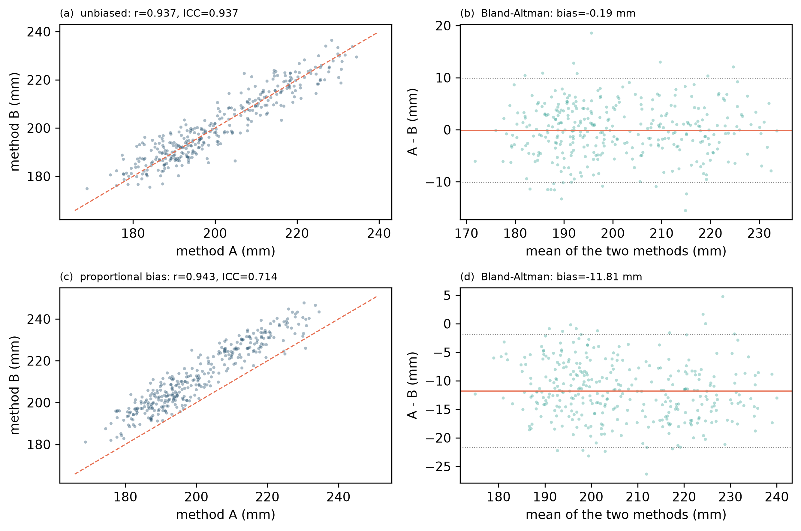
ICC 有十几个变体,差别在于”绝对一致”还是”一致性”、单次还是多次测量、是否有系统偏差。本文用的是 ICC(2,1)(双向随机、绝对一致、单次测量),这个选择必须在方法里写明,否则数字不可比(Shrout & Fleiss,1979)。Lin 的 CCC 与 ICC(2,1) 在这个例子里恰好相等,但它们的定义不同:CCC 直接惩罚均值差与尺度差(Lin,1989)。如果你关心的是”能不能互换”,Bland–Altman 图比任何一个系数都更有信息量(Bland & Altman,1986)。
ICC has a dozen variants, differing in absolute agreement versus consistency, single versus average measurement, and whether systematic bias is modelled. This article uses ICC(2,1) — two-way random, absolute agreement, single measurement — and that choice must be stated or the numbers are not comparable (Shrout & Fleiss, 1979). Lin’s CCC happens to equal ICC(2,1) here, but their definitions differ: CCC directly penalises differences in mean and scale (Lin, 1989). If the question is whether two methods can be interchanged, a Bland–Altman plot carries more information than any single coefficient (Bland & Altman, 1986).
8. 多变量与时序 / Multivariate and time series
RV 系数把两个数据块(\(n\times p\) 与 \(n\times q\))的协方差结构做内积,值域 \([0,1]\);RV2 去掉了对角线上的自相关膨胀,在小 \(p,q\) 时差别明显。CCA 给出两组变量之间的首个正则相关,值域同样是 \([0,1]\),但它对变量的线性组合敏感,且随维度增加而虚高。用企鹅的喙部两块数据算,RV 与 RV2 的差别在小样本下最大。
The RV coefficient takes the inner product of two blocks’ covariance structures (\(n\times p\) and \(n\times q\)) and lies in \([0,1]\); RV2 removes the diagonal inflation of autocorrelation, and the difference is largest for small \(p,q\). CCA gives the first canonical correlation between two blocks, also in \([0,1]\), but it is sensitive to linear combinations and inflates with dimension. On two penguin bill blocks, RV and RV2 differ most in small samples.
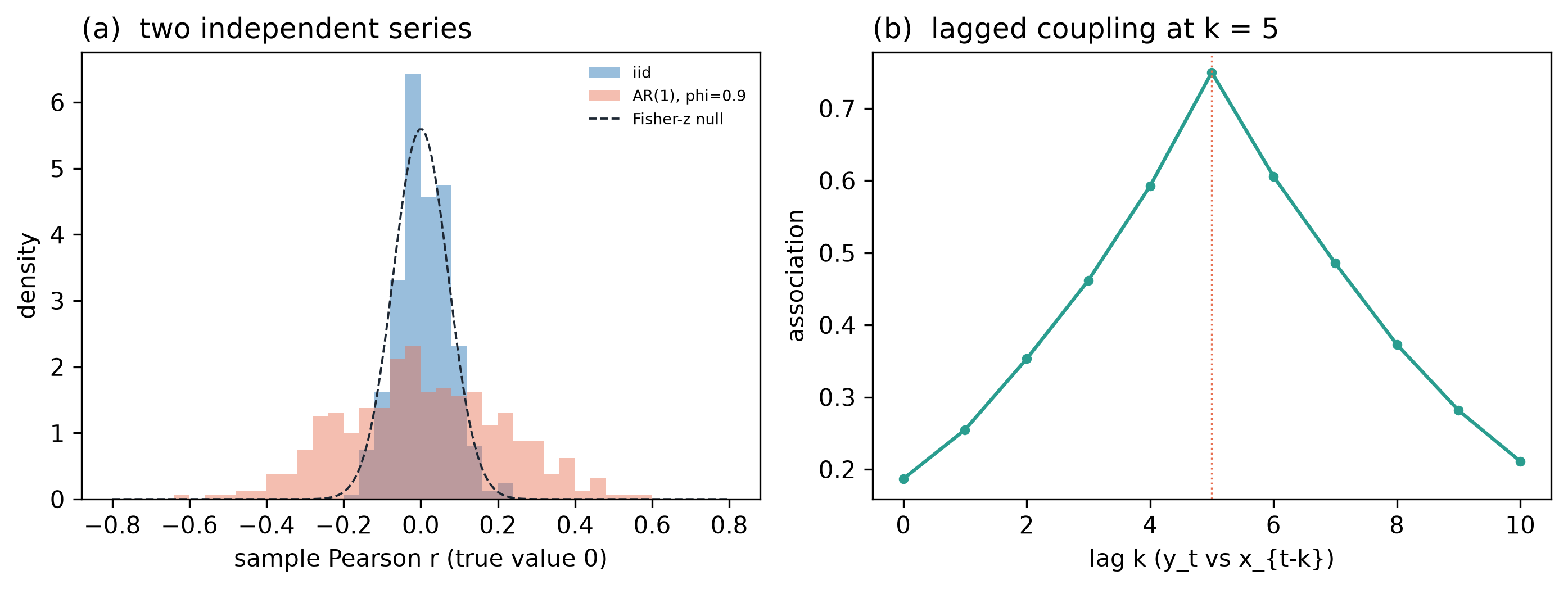
时序要单独说,因为”独立”这个前提在时序里几乎从不成立。两条独立的 AR(1) 序列,\(\phi=0.9\),n = 200,样本 Pearson 的标准差是 0.206,而 iid 情形是 0.068。用 \(|r|>1.96/\sqrt{n}\) 这个规则,假阳性率是 51%,iid 下是 5%;Fisher z 区间的覆盖率是 49%,iid 下 95%。一半以上的”显著相关”是自相关造出来的。
Time series need their own paragraph because the independence premise almost never holds. For two independent AR(1) series with \(\phi=0.9\) and n = 200, the standard deviation of the sample Pearson correlation is 0.206, against 0.068 for iid data. Using the \(|r|>1.96/\sqrt{n}\) rule, the false-positive rate is 51%, against 5% under iid; Fisher-z intervals cover zero 49% of the time, against 95%. More than half of “significant” correlations are manufactured by autocorrelation.
正确的做法不是换一个系数,而是换一个零模型:block bootstrap、相位随机化、或把有效样本量按自相关折减。图 8(b) 展示了另一种情形:当耦合是有滞后的(\(y_t\) 依赖 \(x_{t-5}\)),滞后互相关在 \(k=5\) 处达到峰值 0.75,同时 transfer entropy 从 \(x\) 到 \(y\) 是 0.0261,反向只有 0.0093——方向性只能由这一类有向度量给出。
The right fix is not a different coefficient but a different null model: block bootstrap, phase randomisation, or deflating the effective sample size by the autocorrelation. Figure 8(b) shows the other regime: when the coupling is lagged (\(y_t\) depends on \(x_{t-5}\)), the lagged cross-correlation peaks at \(k=5\) with 0.75, while transfer entropy from \(x\) to \(y\) is 0.0261 against 0.0093 in reverse — direction is something only a directed measure can give.
9. 成本 / Cost
图 9 是单次调用的耗时中位数。Pearson 在 \(n=10^4\) 时仍是 0.08 ms;距离相关在 \(n=2000\) 时 161.4 ms,HSIC 310.4 ms;MIC 在 \(n=5000\) 时 55.5 ms。\(O(n^2)\) 的两个方法在 \(n=2000\) 已经需要几百 MB 的距离矩阵,所以本文没有继续往上测。
Figure 9 shows median time per call. Pearson is still 0.08 ms at \(n=10^4\); distance correlation takes 161.4 ms at \(n=2000\) and HSIC 310.4 ms; MIC takes 55.5 ms at \(n=5000\). The two \(O(n^2)\) methods already need hundreds of megabytes of distance matrix at \(n=2000\), so the grid stops there.
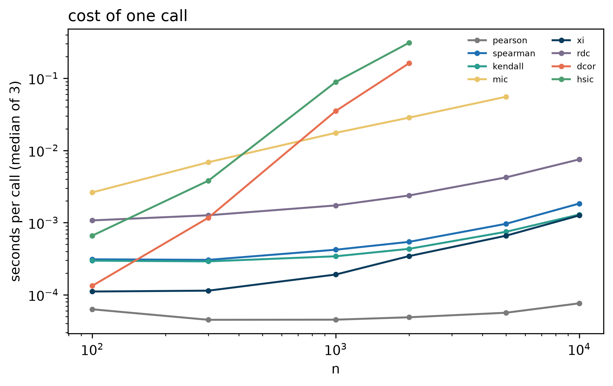
这张图改变的是工作流,而不是结论:如果 \(n=10^5\),omnibus 检验就不该在原始样本上跑,而应先做分箱、抽样或核近似(random Fourier features、Nyström)。“更通用的系数”从来不是免费的。
This figure changes the workflow, not the conclusion: at \(n=10^5\), an omnibus test should not run on the raw sample but on binned, subsampled or kernel-approximated data (random Fourier features, Nyström). “More general” is never free.
10. 怎么选 / Choosing
表 1 是全部 43 个系数的清单。先看中文表,再看英文表;两表行序相同。
Table 1 lists all 43 coefficients. The Chinese table comes first, the English one after it, in the same order.
表 1 四十三个相关系数
| 系数 | 一句话定义 | 零假设 | 不变的变换 | 复杂度 |
|---|---|---|---|---|
| Pearson r | 标准化协方差 | ρ = 0(无线性关联) | 线性 | O(n) |
| 点二列 | 连续变量与 0/1 的 Pearson | 两组均值相等 | 仅二值重编码 | O(n) |
| 偏相关 | 残差化后的 Pearson | 给定 Z 条件独立(线性) | 线性 | O(np²) |
| 半偏相关 | y 与 x 残差的 Pearson | 同上,但只残差化 x | 线性 | O(np²) |
| 多重相关 R | y 与 X 块的复相关 | 所有系数为 0 | 线性 | O(np²) |
| Spearman ρ | 秩上的 Pearson | 无单调关联 | 严格单调 | O(n log n) |
| Spearman footrule | 秩的 L1 距离 | 无秩关联 | 严格单调 | O(n log n) |
| Kendall τ-a | 一致对减不一致对 | 独立(无结) | 严格单调 | O(n²) |
| Kendall τ-b | τ-a 的结校正 | 独立 | 严格单调 | O(n²) |
| Goodman–Kruskal γ | (C−D)/(C+D),忽略结 | 序独立 | 严格单调 | O(n²) |
| Somers’ D | 非对称序关联 | 给定 x 时 y 无单调趋势 | 严格单调 | O(n²) |
| Hoeffding’s D | 经验 copula 与独立的平方偏差 | 独立 | 严格单调 | O(n²) |
| BKR R | 经验 copula 的 omnibus 统计量 | 独立 | 严格单调 | O(n²) |
| distance correlation | 距离协方差的归一化 | 独立 | 旋转、平移、缩放 | O(n²) |
| partial dCor | 去掉 Z 后的 dCor | 给定 Z 条件独立 | 同上 | O(n²) |
| HSIC(归一化) | RKHS 上的协方差 | 独立 | 核的选择 | O(n²) |
| MIC(近似) | 网格上最大归一化 MI | 独立 | 严格单调(理论上) | O(n^1.2) |
| RDC | 随机特征上的线性相关 | 独立 | 线性 | O(n) |
| Chatterjee ξ | 排序后的秩变差 | 独立 | 严格单调(对 x) | O(n log n) |
| ξ(置换校正) | ξ 减去置换偏差 | 独立 | 同上 | O(n log n × B) |
| 互信息 | 联合与边缘的 KL 距离 | 独立 | 严格单调 | O(n + bins²) |
| 归一化 MI | MI / √(HxHy) | 独立 | 严格单调 | 同上 |
| variation of information | Hx + Hy − 2MI | 独立 | 严格单调 | 同上 |
| transfer entropy | 条件 MI,含时间方向 | x 对未来 y 无增量信息 | 严格单调 | O(n × bins³) |
| φ | 2×2 的卡方归一化 | 两二值变量独立 | 行/列置换 | O(n) |
| Cramér’s V | χ²/(n·min(r−1,c−1)) | 分类独立 | 类别重标号 | O(n + rc) |
| Tschuprow’s T | χ² 的几何平均归一化 | 分类独立 | 类别重标号 | O(n + rc) |
| Goodman–Kruskal λ | 预测误差的相对下降 | 给定 x 时 y 的众数不变 | 类别重标号 | O(n + rc) |
| Theil’s U | 条件熵的归一化下降 | 分类独立 | 类别重标号 | O(n + rc) |
| polychoric | 潜在正态下的阈值相关 | 潜在相关为 0 | 单调重编码 | O(n + k²) |
| tetrachoric | 2×2 的 polychoric | 同上 | 同上 | O(n) |
| polyserial | 连续×有序的潜在相关 | 潜在相关为 0 | 单调重编码 | O(n·k) |
| ICC(1,1) | 单向随机效应 | 无组间方差 | 位置与尺度(部分) | O(n) |
| ICC(2,1) | 双向随机、绝对一致 | 无组间方差、无评分者偏差 | 有限 | O(n) |
| Lin’s CCC | 惩罚均值与尺度差的相关系数 | 完全一致 | 仅符号 | O(n) |
| Bland–Altman | 偏倚与一致性界限 | 平均差为 0 | 无 | O(n) |
| RV | 两块协方差的内积 | 两块无关 | 正交变换 | O(n²p + n²q) |
| RV2 | 去掉对角膨胀的 RV | 同上 | 同上 | 同上 |
| CCA(首正则) | 两块的最佳线性组合相关 | 无正则相关 | 块内线性变换 | O(np² + nq²) |
| cdCor(滞后 dCor 代理) | 时序的距离相关 | 两序列独立 | 平移 | O(n² × lags) |
| 滞后互相关 | 滞后上的最大绝对相关 | 无滞后关联 | 平移 | O(n × lags) |
| Rényi 最大相关 | 最优变换后的相关上确界 | 独立 | 严格单调 | 理论量 |
| copula 视角的 Spearman | 12∫(C−uv) du dv | 独立 | 严格单调 | 理论量 |
English
Table 1 Forty-three coefficients
| Coefficient | Definition | H0 | Invariant to | Cost |
|---|---|---|---|---|
| Pearson r | standardised covariance | ρ = 0 (no linear association) | linear | O(n) |
| point-biserial | Pearson with a 0/1 code | equal group means | binary recoding | O(n) |
| partial r | Pearson of residuals | conditional independence (linear) | linear | O(np²) |
| semi-partial r | y against residualised x | as above, x only | linear | O(np²) |
| multiple R | correlation of y with a block | all coefficients zero | linear | O(np²) |
| Spearman ρ | Pearson on ranks | no monotone association | strictly monotone | O(n log n) |
| Spearman footrule | L1 distance of ranks | no rank association | strictly monotone | O(n log n) |
| Kendall τ-a | concordant minus discordant | independence (no ties) | strictly monotone | O(n²) |
| Kendall τ-b | tie-corrected τ-a | independence | strictly monotone | O(n²) |
| Goodman–Kruskal γ | (C−D)/(C+D), ties ignored | independence of order | strictly monotone | O(n²) |
| Somers’ D | asymmetric ordinal association | no monotone trend of y on x | strictly monotone | O(n²) |
| Hoeffding’s D | squared deviation of the empirical copula | independence | strictly monotone | O(n²) |
| BKR R | omnibus statistic on the empirical copula | independence | strictly monotone | O(n²) |
| distance correlation | normalised distance covariance | independence | rotation, translation, scaling | O(n²) |
| partial dCor | dCor after removing Z | conditional independence | as above | O(n²) |
| HSIC (normalised) | covariance in an RKHS | independence | choice of kernel | O(n²) |
| MIC (approximate) | maximal normalised MI over grids | independence | strictly monotone (in theory) | O(n^1.2) |
| RDC | linear correlation of random features | independence | linear | O(n) |
| Chatterjee ξ | rank variation after sorting | independence | strictly monotone in x | O(n log n) |
| ξ (permutation-corrected) | ξ minus its permutation bias | independence | as above | O(n log n × B) |
| mutual information | KL divergence of joint and marginals | independence | strictly monotone | O(n + bins²) |
| normalised MI | MI / √(HxHy) | independence | strictly monotone | as above |
| variation of information | Hx + Hy − 2MI | independence | strictly monotone | as above |
| transfer entropy | conditional MI with time direction | x adds nothing about future y | strictly monotone | O(n × bins³) |
| φ | chi-square normalisation of a 2×2 table | independence of two binaries | row/column permutation | O(n) |
| Cramér’s V | χ²/(n·min(r−1,c−1)) | categorical independence | relabelling | O(n + rc) |
| Tschuprow’s T | geometric-mean normalisation of χ² | categorical independence | relabelling | O(n + rc) |
| Goodman–Kruskal λ | proportional reduction in prediction error | the mode of y is unchanged by x | relabelling | O(n + rc) |
| Theil’s U | normalised drop in conditional entropy | categorical independence | relabelling | O(n + rc) |
| polychoric | threshold correlation under latent normality | latent correlation zero | monotone recoding | O(n + k²) |
| tetrachoric | polychoric for 2×2 | as above | as above | O(n) |
| polyserial | latent correlation, continuous × ordinal | latent correlation zero | monotone recoding | O(n·k) |
| ICC(1,1) | one-way random effects | no between-subject variance | location and scale (partly) | O(n) |
| ICC(2,1) | two-way random, absolute agreement | no subject or rater effects | limited | O(n) |
| Lin’s CCC | correlation penalising mean and scale | perfect agreement | sign only | O(n) |
| Bland–Altman | bias and limits of agreement | mean difference zero | none | O(n) |
| RV | inner product of two covariance blocks | the blocks are unrelated | orthogonal transforms | O(n²p + n²q) |
| RV2 | diagonal-free RV | as above | as above | as above |
| CCA (first canonical) | best linear combinations of two blocks | no canonical correlation | linear within blocks | O(np² + nq²) |
| cdCor (lagged dCor proxy) | distance correlation for series | the series are independent | shift | O(n² × lags) |
| lagged cross-correlation | largest absolute correlation over lags | no lagged association | shift | O(n × lags) |
| Rényi maximal correlation | sup over transforms | independence | strictly monotone | theoretical |
| copula Spearman identity | 12∫(C−uv) du dv | independence | strictly monotone | theoretical |
表 2 按数据类型给建议。它不是算法,而是一张”先问什么”的清单。
Table 2 maps data types to recommendations. It is not an algorithm but a checklist of what to ask first.
表 2 按数据类型选系数
| 数据 / 问题 | 首选 | 备选 | 不要用 |
|---|---|---|---|
| 连续、近似线性 | Pearson | Spearman(稳健性检查) | MIC(小样本) |
| 连续、单调非线性 | Spearman、Kendall | ξ、polyserial(若有潜在变量) | Pearson |
| 任意依赖、n 较小 | dCor、HSIC | MIC(注明近似) | Pearson、Spearman |
| 任意依赖、n 较大 | MIC、ξ、RDC | 分箱后的 MI | 原始 dCor(\(O(n^2)\)) |
| 有序(Likert) | polychoric、Kendall τ-b | Spearman | Pearson |
| 二值 × 连续 | 点二列 | 逻辑回归系数 | Pearson 直接套 |
| 分类 × 分类 | Cramér’s V、Theil’s U | λ | Pearson |
| 两方法是否可互换 | Bland–Altman、ICC(2,1)、CCC | —— | Pearson |
| 多变量两块 | RV2、CCA | RV | 逐对 Pearson |
| 时间序列 | 滞后互相关、transfer entropy | cdCor | iid 的 Fisher-z |
| 有混杂 | 偏相关、dCor 偏版本 | 分层分析 | 边际 Pearson |
English
Table 2 Choosing by data type
| Data / question | First choice | Alternative | Avoid |
|---|---|---|---|
| continuous, roughly linear | Pearson | Spearman (robustness check) | MIC at small n |
| continuous, monotone nonlinear | Spearman, Kendall | ξ, polyserial with a latent variable | Pearson |
| arbitrary dependence, small n | dCor, HSIC | MIC (labelled approximate) | Pearson, Spearman |
| arbitrary dependence, large n | MIC, ξ, RDC | binned MI | raw dCor (\(O(n^2)\)) |
| ordinal (Likert) | polychoric, Kendall τ-b | Spearman | Pearson |
| binary × continuous | point-biserial | logistic coefficient | Pearson applied blindly |
| categorical × categorical | Cramér’s V, Theil’s U | λ | Pearson |
| are two methods interchangeable | Bland–Altman, ICC(2,1), CCC | —— | Pearson |
| two multivariate blocks | RV2, CCA | RV | pairwise Pearson |
| time series | lagged cross-correlation, transfer entropy | cdCor | iid Fisher-z |
| confounding present | partial r, partial dCor | stratified analysis | marginal Pearson |
表 3 是本文的实测汇总。它只包含可以比较的列:同一批零分布、同一批数据生成器。
Table 3 summarises the measurements. It only contains comparable columns: one null protocol and one data generator.
表 3 实测:功效、异常值与成本
| 系数 | 线性(n=100) | 圆(n=300) | 20% 污染后保留 | n=2000 耗时 |
|---|---|---|---|---|
| Pearson | 1.00 | 0.03 | 6% | 0.05 ms |
| Spearman | 1.00 | 0.03 | 65% | 0.54 ms |
| Kendall τ-b | 1.00 | 0.00 | 65% | 0.43 ms |
| dCor | 1.00 | 1.00 | 20% | 161.4 ms |
| HSIC | 1.00 | 1.00 | —— | 310.4 ms |
| MIC | 1.00 | 1.00 | 79% | 28.5 ms |
| RDC | 1.00 | 0.03 | —— | 2.38 ms |
| ξ | 1.00 | 1.00 | 81% | 0.34 ms |
English
Table 3 Measured power, robustness and cost
| Coefficient | linear (n=100) | circle (n=300) | retained under 20% contamination | time at n=2000 |
|---|---|---|---|---|
| Pearson | 1.00 | 0.03 | 6% | 0.05 ms |
| Spearman | 1.00 | 0.03 | 65% | 0.54 ms |
| Kendall τ-b | 1.00 | 0.00 | 65% | 0.43 ms |
| dCor | 1.00 | 1.00 | 20% | 161.4 ms |
| HSIC | 1.00 | 1.00 | —— | 310.4 ms |
| MIC | 1.00 | 1.00 | 79% | 28.5 ms |
| RDC | 1.00 | 0.03 | —— | 2.38 ms |
| ξ | 1.00 | 1.00 | 81% | 0.34 ms |
最后是误用清单。它比任何一张表都更常被用到。
Finally, the misuse list. It gets used more often than any table.
| 误用 / Misuse | 为什么错 / Why it is wrong |
|---|---|
| 用 Pearson 比较两个数据集的”相关强度” / comparing Pearson across datasets | 受量纲、range restriction 与选择偏差影响 / affected by scale, range restriction and selection |
| 把 \(r^2\) 当作”解释了多少” / reading \(r^2\) as variance explained | 只在简单线性回归里成立,且不区分方向 / only in simple linear regression |
| 用 Pearson 判断一致性 / using Pearson for agreement | 对系统偏差完全不敏感 / blind to systematic bias |
| 对有序变量用 Pearson / Pearson on ordinal data | 分箱衰减,方向依赖编码 / attenuation, coding-dependent |
| 直接对时序做 Fisher z / Fisher-z on time series | 有效样本量被高估,假阳性可过半 / effective n is inflated |
| 在混杂存在时报告边际相关 / reporting marginal r under confounding | 可能连符号都错 / even the sign can flip |
| 用同一个 r 比较不同 n 的 MIC / comparing MIC across n | 受 \(B(n)\) 限制 / bounded by \(B(n)\) |
| 把”不显著”读成”无关” / reading non-significance as independence | 功效不足与真无关不可区分 / low power mimics independence |
English
| Misuse | Why it is wrong |
|---|---|
| comparing Pearson across datasets | affected by scale, range restriction and selection |
| reading \(r^2\) as variance explained | only valid in simple linear regression, and direction is lost |
| using Pearson for agreement | blind to systematic bias |
| Pearson on ordinal data | attenuation, and the value depends on the coding |
| Fisher-z on time series | the effective sample size is inflated; false positives can exceed half |
| reporting marginal r under confounding | even the sign can flip |
| comparing MIC across sample sizes | bounded by \(B(n)\) |
| reading non-significance as independence | low power is indistinguishable from true independence |
11. 方法与局限 / Methods and limits
- 实现:全部系数在
experiments/common/corr.py中从零实现,只依赖 NumPy/SciPy;Pearson、Spearman、Kendall 与 SciPy 的结果对拍一致,其余用已知极限(独立的 dCor ≈ 0、\(y=x\) 的 \(\xi\approx 1\)、\(y=x^2\) 的 \(\xi\approx 1\))自检。
Implementation: every coefficient is written from scratch inexperiments/common/corr.pywith NumPy/SciPy only; Pearson, Spearman and Kendall agree with SciPy, and the rest were checked against known limits (dCor ≈ 0 under independence, \(\xi\approx 1\) for \(y=x\) and \(y=x^2\)). - 校准:每个(方法,n,零数据)用 400 次抽样估计 95% 分位,再用 400 次新抽样估计拒绝率;蒙特卡洛标准误约 1.1 个百分点。
Calibration: 400 draws for the 95th percentile and 400 fresh draws for the rejection rate per cell; the Monte-Carlo standard error is about 1.1 percentage points. - 功效:零分布由在每个抽样内置换 \(y\) 得到(200 次),功效由 60 次独立抽样估计;因此表中的功效有 ±6% 左右的不确定度。
Power: the null permutes \(y\) within each draw (200 permutations) and power uses 60 independent draws, so each cell carries roughly ±6% uncertainty. - 未做的事:没有做多变量 omnibus(如 dCov 的块版本)的功效比较;没有对 MIC 做 \(B(n)\) 之外的偏差校正;没有用真实的高维组学数据检验 RV/CCA;没有给 \(\xi\) 的置信区间。
Not done: no power comparison for multivariate omnibus tests; no bias correction for MIC beyond \(B(n)\); no real high-dimensional omics test of RV/CCA; no confidence intervals for \(\xi\). - 不能说的话:本文没有证明任何一个系数”最好”,也没有证明 omnibus 检验在所有场景下优于线性相关。它证明的是一组更窄的命题:不同系数的零假设不同、不变性不同、功效分布不同,而这些差异可以在同一批数据上被测量出来。
What cannot be said: nothing here shows that any coefficient is “best”, nor that omnibus tests dominate linear correlation everywhere. What it shows is narrower: the null hypotheses differ, the invariances differ and the power profiles differ, and those differences can be measured on one dataset.
八个脚本都在本目录:01_calibration.py(校准)、02_power.py(功效)、03_invariance.py(单调变换与污染)、04_same_r.py(Anscombe 与 Datasaurus)、05_agreement.py(一致性)、06_confound.py(混杂与辛普森)、07_timeseries.py(时序)、08_complexity.py(成本)。重跑任一脚本即可复现对应的数字与图。
Scripts sit in this directory: 01_calibration.py (calibration), 02_power.py (power), 03_invariance.py (monotone transforms and contamination), 04_same_r.py (Anscombe and Datasaurus), 05_agreement.py (agreement), 06_confound.py (confounding and Simpson), 07_timeseries.py (time series) and 08_complexity.py (cost). Rerun any of them to reproduce the corresponding numbers and figures.
参考文献 / References
- Anscombe, F. J. (1973). Graphs in statistical analysis. The American Statistician 27, 17–21. doi:10.1080/00031305.1973.10478966
- Székely, G. J., Rizzo, M. L., & Bakirov, N. K. (2007). Measuring and testing dependence by correlation of distances. Annals of Statistics 35, 2769–2794. doi:10.1214/009053607000000505
- Székely, G. J., & Rizzo, M. L. (2014). Partial distance correlation with methods for dissimilarities. Annals of Statistics 42, 2382–2412. doi:10.1214/14-AOS1255
- Gretton, A., Bousquet, O., Smola, A., & Schölkopf, B. (2005). Measuring statistical dependence with Hilbert–Schmidt norms. Algorithmic Learning Theory, 63–77. doi:10.1007/11564089_7
- Reshef, D. N., et al. (2011). Detecting novel associations in large data sets. Science 334, 1518–1524. doi:10.1126/science.1205438
- Simon, N., & Tibshirani, R. (2014). Comment on “Detecting novel associations in large data sets”. Science 346, 315. arXiv:1401.7645
- Chatterjee, S. (2021). A new coefficient of correlation. Journal of the American Statistical Association 116, 2009–2022. doi:10.1080/01621459.2020.1758115
- Lopez-Paz, D., Hennig, P., & Schölkopf, B. (2013). The randomized dependence coefficient. Advances in Neural Information Processing Systems 26.
- Hoeffding, W. (1948). A non-parametric test of independence. Annals of Mathematical Statistics 19, 546–557. doi:10.1214/aoms/1177730150
- Blum, J. R., Kiefer, J., & Rosenblatt, M. (1961). Distribution free tests of independence based on the sample distribution function. Annals of Mathematical Statistics 32, 485–498. doi:10.1214/aoms/1177705055
- Goodman, L. A., & Kruskal, W. H. (1954). Measures of association for cross classifications. JASA 49, 732–764. doi:10.1080/01621459.1954.10501231
- Somers, R. H. (1962). A new asymmetric measure of association for ordinal variables. American Sociological Review 27, 799–811. doi:10.2307/2090408
- Kendall, M. G. (1938). A new measure of rank correlation. Biometrika 30, 81–93. doi:10.1093/biomet/30.1-2.81
- Spearman, C. (1904). The proof and measurement of association between two things. American Journal of Psychology 15, 72–101. doi:10.2307/1412159
- Diaconis, P., & Graham, R. L. (1977). Spearman’s footrule as a measure of disarray. JRSS-B 39, 262–268. doi:10.1111/j.2517-6161.1977.tb01624.x
- Shannon, C. E. (1948). A mathematical theory of communication. Bell System Technical Journal 27, 379–423. doi:10.1002/j.1538-7305.1948.tb01338.x
- Kraskov, A., Stögbauer, H., & Grassberger, P. (2004). Estimating mutual information. Physical Review E 69, 066138. doi:10.1103/PhysRevE.69.066138
- Schreiber, T. (2000). Measuring information transfer. Physical Review Letters 85, 461–464. doi:10.1103/PhysRevLett.85.461
- Cramér, H. (1946). Mathematical Methods of Statistics. Princeton University Press.
- Theil, H. (1970). On the estimation of relationships involving qualitative variables. American Journal of Sociology 76, 103–154. doi:10.1086/224909
- Olsson, U. (1979). Maximum likelihood estimation of the polychoric correlation coefficient. Psychometrika 44, 443–460. doi:10.1007/BF02296262
- Drasgow, F. (1986). Polychoric and polyserial correlations. In Encyclopedia of Statistical Sciences 7, 68–74. Wiley.
- Shrout, P. E., & Fleiss, J. L. (1979). Intraclass correlations: uses in assessing rater reliability. Psychological Bulletin 86, 420–428. doi:10.1037/0033-2909.86.2.420
- Lin, L. I.-K. (1989). A concordance correlation coefficient to evaluate reproducibility. Biometrics 45, 255–268. doi:10.2307/2532051
- Bland, J. M., & Altman, D. G. (1986). Statistical methods for assessing agreement between two methods of clinical measurement. The Lancet 327, 307–310. doi:10.1016/S0140-6736(86)90837-8
- Escoufier, Y. (1973). Le traitement des variables vectorielles. Biometrics 29, 751–760. doi:10.2307/2529140
- Hotelling, H. (1936). Relations between two sets of variates. Biometrika 28, 321–377. doi:10.1093/biomet/28.3-4.321
- Fisher, R. A. (1921). On the “probable error” of a coefficient of correlation deduced from a small sample. Metron 1, 3–32.
- Rényi, A. (1959). On measures of dependence. Acta Mathematica Academiae Scientiarum Hungaricae 10, 441–451. doi:10.1007/BF02024507
- Nelsen, R. B. (2006). An Introduction to Copulas, 2nd ed. Springer.
- Wolfram, S. (2002). A New Kind of Science. Wolfram Media.
以上条目中,期刊论文给出 DOI;图书与会议论文集给出出版社或卷期;预印本给出 arXiv 编号。凡本文未能独立核实的 DOI,一律未写,只保留期刊卷页。数值实现与数据来源见 experiments/README.md。
Journal articles above carry DOIs; books and proceedings carry publisher or volume information; the preprint carries an arXiv identifier. Any DOI that could not be independently checked is omitted, leaving only journal, volume and pages. Implementation and data provenance are in experiments/README.md.